Extracting Crop Pixels from Dynamic World V1 using Google Earth Engine

Data Setup

We’ll start by loading the necessary datasets: the H3 hexagon grid for Pakistan and the Dynamic World V1 image collection for the year 2023. Filtering will be applied to focus on the region of interest and time frame.

var pak = ee.FeatureCollection("projects/ee-mohsin1570/assets/Pak_H3_R6");

// Load the Dynamic World ImageCollection for 2023, filtered by geographic boundary
var dynamicWorld2023 = ee.ImageCollection('GOOGLE/DYNAMICWORLD/V1')
                    .filterBounds(pak)
                    .filterDate('2023-01-01', '2023-12-31');

Next, we’ll clip the dataset to the boundaries of Pakistan to limit the analysis to the desired region.

// Clip each image in the collection to Pakistan's boundary
var dynamicWorld2023 = dynamicWorld2023.map(function(image) {
  return image.clip(pak);
});

Filtering Crop Pixels

Our focus is on identifying crop pixels with high confidence. We’ll use a probability threshold of 50%, meaning only pixels classified as crops with a confidence level greater than or equal to 50% will be retained. Additionally, we’ll impose a temporal threshold, requiring pixels to be classified as crops for more than 50% of the time in 2023.

• Advantages of these thresholds:
  • 50% confidence threshold: This is a moderate cutoff, ensuring that the majority of crop predictions are reasonably certain without being overly restrictive. It captures a wider set of potential crop pixels, which is useful in areas with fluctuating land cover types.
  • 50% temporal threshold: This ensures consistency in crop classification, which is particularly useful for areas with seasonal crops. It reduces the likelihood of transient misclassifications affecting the analysis.

// Apply the crop confidence threshold (50%)
var threshold = 0.5;

// Filter pixels classified as crops with >50% confidence
var cropsMasked = dynamicWorld2023.map(function(image) {
  var cropsBand = image.select('crops');
  return cropsBand.updateMask(cropsBand.gte(threshold));
});

// Count the number of times each pixel is classified as crop
var cropCount = cropsMasked.reduce(ee.Reducer.sum());

// Get the total number of images in the collection
var totalImages = cropsMasked.size();

// Apply temporal threshold: crop >50% of the year
var majorityThreshold = totalImages.multiply(0.5);
var majorityCrops = cropCount.gte(majorityThreshold);

Visualizing the Results

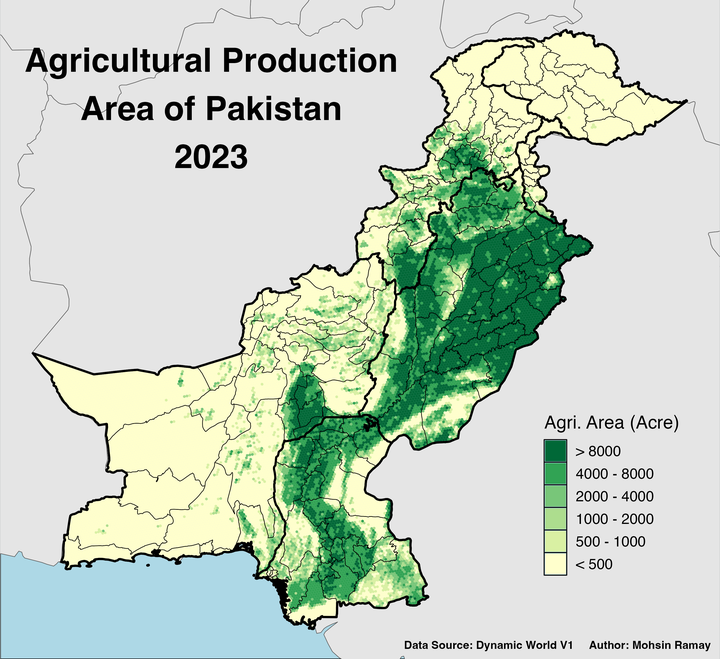
After filtering, it’s important to visualize the spatial distribution of crop pixels to validate the results. This can be done by adding the processed data to the Google Earth Engine map interface.

// Visualize the crop pixels
Map.addLayer(majorityCrops, {min: 0, max: 1, palette: ['orange']}, 'Majority Crops in 2023');
Map.centerObject(pak, 5);

Aggregating Data to H3 Hexagons

Once we’ve filtered and visualized the crop pixels, we can aggregate the data to the H3 hexagon grid. This step is essential for reducing the complexity of the high-resolution raster data and facilitating large-scale analysis.

// Count crop pixels in each hexagon
var cropPixelCount = majorityCrops.reduceRegions({
  collection: pak,
  reducer: ee.Reducer.sum(),
  scale: 10  
});

Exporting Results

// Export hexagon-level crop pixel count as GeoJSON
Export.table.toDrive({
  collection: cropPixelCount,
  description: 'CropPixelCount_Hexagons',
  fileFormat: 'GeoJSON',
  folder: 'Remote Sensing',
  fileNamePrefix: 'crop_pixel_count'  
});

// Export the majority crops raster as GeoTIFF
Export.image.toDrive({
  image: majorityCrops,
  description: 'MajorityCrops_Resampled_10m',
  fileNamePrefix: 'crops_resampled_10m',
  scale: 10,  // The resolution in meters
  region: pak.geometry(),
  crs: 'EPSG:4326',
  maxPixels: 1e13,
  fileFormat: 'GeoTIFF',
  formatOptions: {
    cloudOptimized: true
  },
  folder: 'Remote Sensing'
});

Conclusion

In this post, we successfully demonstrated how to extract crop pixels from the Dynamic World V1 dataset using Google Earth Engine. By applying confidence and temporal thresholds, we ensured that only consistent and reliable crop classifications were included. The data was then aggregated to H3 hexagons for large-scale analysis and exported in both vector and raster formats. This approach is flexible and can be extended to other land cover types such as forests or urban areas.

Stay tuned for further insights on using Google Earth Engine for large-scale remote sensing applications.

That’s it!

Feel free to reach me out if you got any questions.