Mapping Cropping Area in Pakistan: A Professional Approach

Last updated on Oct 4, 2024 7 min read Geospatial Analysis

This blog post continues from my previous post where I demonstrated how to extract and download crop pixels from the Dynamic World V1 dataset using Google Earth Engine.

In this post, we will utilize the downloaded data of pixel counts in each H3 hexagon to calculate the agricultural production area in hectares or acres and visualize these results in a spatial map.

Loading Required Libraries

Before proceeding with the analysis, we load the necessary libraries. We use tidyverse for data manipulation, sf for handling spatial data, and rnaturalearth for loading country boundary data.

library(tidyverse)
library(sf)
library(rnaturalearth)

Loading Data

Next, we load the dataset of agricultural areas for Pakistan. The dataset is stored in a GeoJSON format and read using the st_read function from the sf package.

# Load the dataset of cropping area
agri_area <- st_read("../data/crop_area/crop_area_2023.geojson")

## Reading layer `crop_area_2023_new' from data source 
##   `/Users/muhammadmohsinraza/Downloads/DataWim/content/post/data/crop_area/crop_area_2023.geojson' 
##   using driver `GeoJSON'
## Simple feature collection with 22977 features and 5 fields
## Geometry type: POLYGON
## Dimension:     XY
## Bounding box:  xmin: 60.91898 ymin: 23.69942 xmax: 77.77897 ymax: 37.09376
## Geodetic CRS:  WGS 84

head(agri_area)

## Simple feature collection with 6 features and 5 fields
## Geometry type: POLYGON
## Dimension:     XY
## Bounding box:  xmin: 67.23219 ymin: 23.69942 xmax: 68.21128 ymax: 24.51154
## Geodetic CRS:  WGS 84
##          h3_index pixels  area  h3_area    prop_area
## 1 8642e2107ffffff    181 18100 34427821 5.257376e-04
## 2 8642e211fffffff    495 49500 34399715 1.438965e-03
## 3 8642e210fffffff    109 10900 34439096 3.165008e-04
## 4 8642e2117ffffff    244 24400 34388407 7.095415e-04
## 5 8642e6ab7ffffff      4   400 34842431 1.148026e-05
## 6 8642e6b9fffffff     82  8200 34869130 2.351650e-04
##                         geometry
## 1 POLYGON ((68.07787 23.79259...
## 2 POLYGON ((68.11966 23.75048...
## 3 POLYGON ((68.14121 23.80159...
## 4 POLYGON ((68.05637 23.74149...
## 5 POLYGON ((67.27489 24.44891...
## 6 POLYGON ((67.23219 24.49114...

Loading Country Boundary Lines

We also load shapefiles representing administrative boundaries of Pakistan at different levels. These boundary lines will be used to enhance the visualization of the agricultural area.

# Load boundary shapefiles
pak0 <- st_read("../data/shapefiles/pak_admbnda_adm0_wfp_20220909.shp")

## Reading layer `pak_admbnda_adm0_wfp_20220909' from data source 
##   `/Users/muhammadmohsinraza/Downloads/DataWim/content/post/data/shapefiles/pak_admbnda_adm0_wfp_20220909.shp' 
##   using driver `ESRI Shapefile'
## Simple feature collection with 1 feature and 10 fields
## Geometry type: MULTIPOLYGON
## Dimension:     XY
## Bounding box:  xmin: 60.8786 ymin: 23.69468 xmax: 77.83397 ymax: 37.08942
## Geodetic CRS:  WGS 84

pak1 <- st_read("../data/shapefiles/pak_admbnda_adm1_wfp_20220909.shp")

## Reading layer `pak_admbnda_adm1_wfp_20220909' from data source 
##   `/Users/muhammadmohsinraza/Downloads/DataWim/content/post/data/shapefiles/pak_admbnda_adm1_wfp_20220909.shp' 
##   using driver `ESRI Shapefile'
## Simple feature collection with 7 features and 12 fields
## Geometry type: MULTIPOLYGON
## Dimension:     XY
## Bounding box:  xmin: 60.8786 ymin: 23.69468 xmax: 77.83397 ymax: 37.08942
## Geodetic CRS:  WGS 84

pak2 <- st_read("../data/shapefiles/pak_admbnda_adm2_wfp_20220909.shp")

## Reading layer `pak_admbnda_adm2_wfp_20220909' from data source 
##   `/Users/muhammadmohsinraza/Downloads/DataWim/content/post/data/shapefiles/pak_admbnda_adm2_wfp_20220909.shp' 
##   using driver `ESRI Shapefile'
## Simple feature collection with 160 features and 14 fields
## Geometry type: MULTIPOLYGON
## Dimension:     XY
## Bounding box:  xmin: 60.8786 ymin: 23.69468 xmax: 77.83397 ymax: 37.08942
## Geodetic CRS:  WGS 84

# Plot the boundary lines
plot(st_geometry(pak2), border = "gray")
plot(st_geometry(pak1), add = TRUE, size = 1, border = "blue")
plot(st_geometry(pak0), add = TRUE, lwd = 2, border = "black")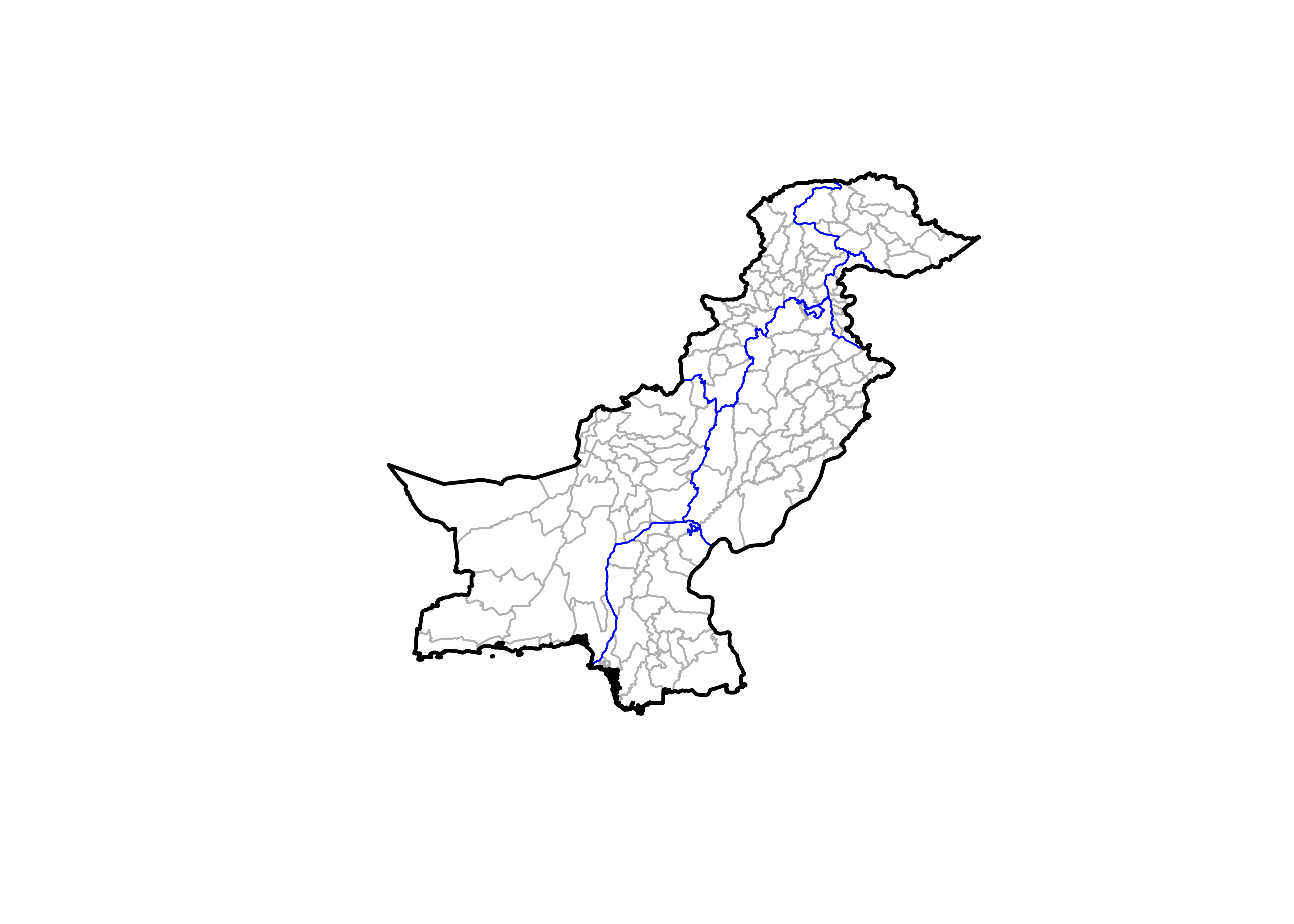

Loading World Countries Boundary Data

Finally, we load the boundary data for countries in Asia using the rnaturalearth package. This will help provide context in the map by displaying neighboring countries.

# Load countries boundary data for Asia
world <- ne_countries(scale = 50, type = "countries", continent = "Asia", returnclass = "sf")

Data Processing

To estimate the agricultural area in different units, we need to calculate the area based on the pixel count. Since the resolution of the Dynamic World V1 dataset is 10 meters, the area calculations can be derived accordingly.

Area Calculation

The following code calculates the area in square meters, hectares, and acres.

# Calculate area in square meters, hectares, and acres
agri_area <- agri_area |> 
  mutate(
    area = pixels * 10 * 10,    # Area in square meters
    area_ha = area / 10000,     # Area in hectares
    area_ac = area_ha * 2.471   # Area in acres
  )

head(agri_area)

## Simple feature collection with 6 features and 7 fields
## Geometry type: POLYGON
## Dimension:     XY
## Bounding box:  xmin: 67.23219 ymin: 23.69942 xmax: 68.21128 ymax: 24.51154
## Geodetic CRS:  WGS 84
##          h3_index pixels  area  h3_area    prop_area
## 1 8642e2107ffffff    181 18100 34427821 5.257376e-04
## 2 8642e211fffffff    495 49500 34399715 1.438965e-03
## 3 8642e210fffffff    109 10900 34439096 3.165008e-04
## 4 8642e2117ffffff    244 24400 34388407 7.095415e-04
## 5 8642e6ab7ffffff      4   400 34842431 1.148026e-05
## 6 8642e6b9fffffff     82  8200 34869130 2.351650e-04
##                         geometry area_ha  area_ac
## 1 POLYGON ((68.07787 23.79259...    1.81  4.47251
## 2 POLYGON ((68.11966 23.75048...    4.95 12.23145
## 3 POLYGON ((68.14121 23.80159...    1.09  2.69339
## 4 POLYGON ((68.05637 23.74149...    2.44  6.02924
## 5 POLYGON ((67.27489 24.44891...    0.04  0.09884
## 6 POLYGON ((67.23219 24.49114...    0.82  2.02622

Exploratory Data Analysis (EDA)

We can visualize the distribution of agricultural area in both units (hectares and acres). This helps us understand the general pattern of land coverage across different regions.

# Visualize the distribution of agricultural area
agri_area |> 
  as.data.frame() |> 
  pivot_longer(names_to = "Area", values_to = "value", cols = c(area_ha, area_ac)) |> 
  ggplot(aes(x = value)) +
  geom_histogram(bins = 30, fill = "steelblue", color = "white") +  # Improved visualization
  theme_bw(base_size = 14) +
  facet_wrap(~Area, scales = "free") +
  labs(
    title = "Distribution of Agricultural Area in Pakistan",
    x = "Area",
    y = "Frequency"
  )

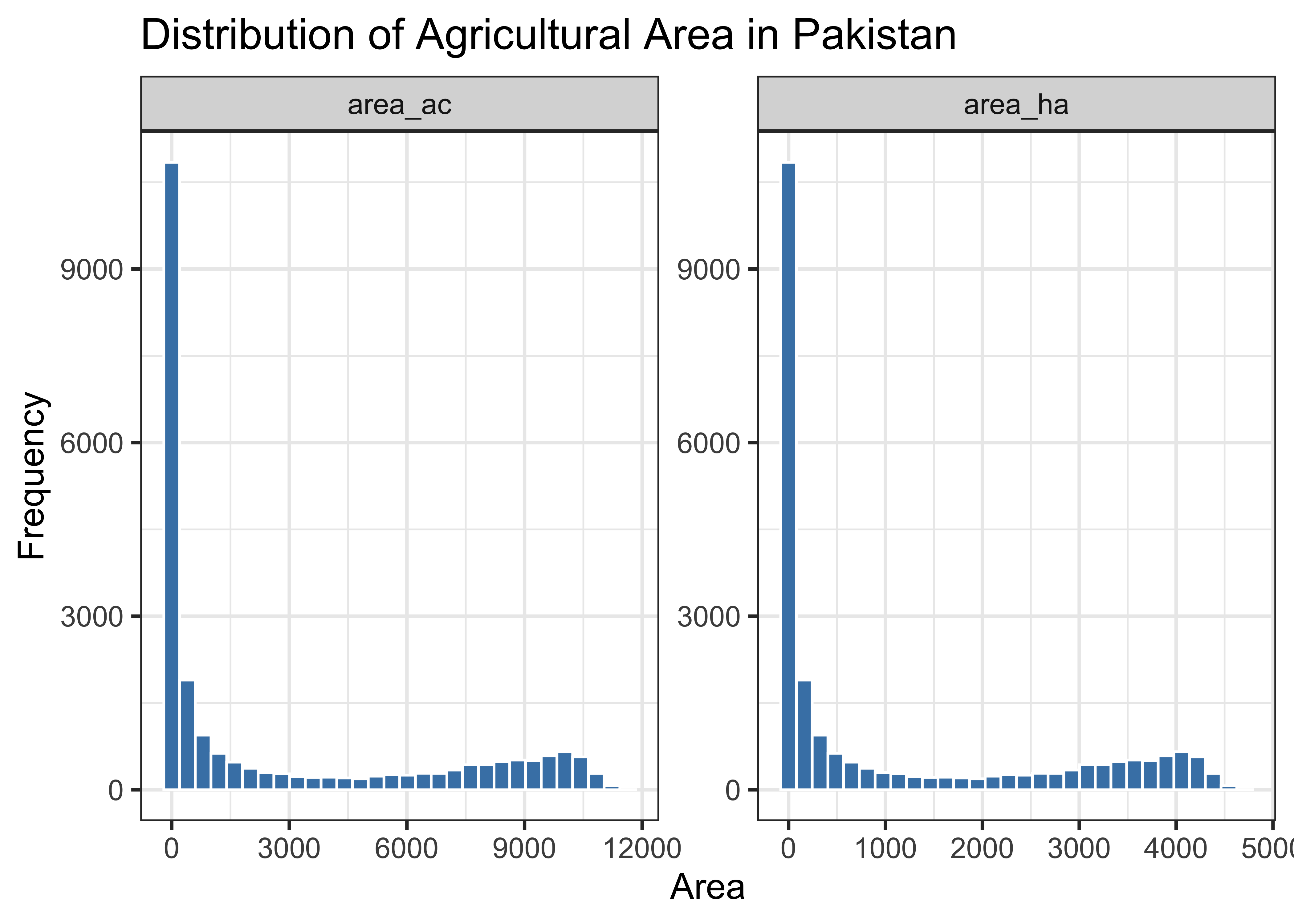
The histogram reveals a strong right-skewed trend, indicating that the majority of H3 hexagons have minimal or no agricultural area. This clustering effect is typical, as agricultural regions tend to be concentrated in specific parts of the country.

Mapping Agricultural Area

Defining Breaks for Area Intervals

To visualize the data effectively, we need to define categories for the agricultural area. In this map, we will focus on visualizing the area in acres. I have defined the bins based on empirical observations, but these can be adjusted as per the requirements of the study.

# Define breaks for intervals
breaks <- c(-Inf, 500, 1000, 2000, 4000, 8000, Inf)

agri_area <- agri_area |> 
  mutate(interval = cut(area_ac, breaks = breaks, labels = c("< 500", "500 - 1000", "1000 - 2000", "2000 - 4000", "4000 - 8000", "> 8000")))

Creating the Spatial Map

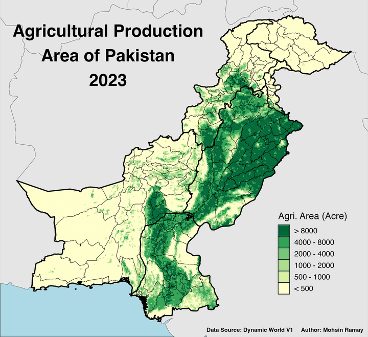
The map below visualizes the cropping area in Pakistan using a color-coded approach to represent different area intervals.

# Define the base map with cropping areas
pp <- ggplot() +
  theme_void(base_size = 14) +
  xlim(60.8786, 77.83397) +
  ylim(23.69468, 37.08942) +
  geom_sf(data = world) +
  geom_sf(data = agri_area, aes(fill = interval), color = NA) +
  scale_fill_brewer(palette = "YlGn", direction = 1) +
  guides(fill = guide_legend(reverse = TRUE)) +
  geom_sf(data = pak2, fill = NA, color = "black") +
  geom_sf(data = pak1, fill = NA, color = "black", linewidth = 0.75) +
    geom_sf(data = pak0, fill = NA, color = "black", linewidth = 0.8) +
  theme(
    panel.background = element_rect(fill = "lightblue"),
    legend.position = c(0.85, 0.25)
  ) +
  annotate("text", x = 65.5, y = 34, hjust = 0.5, vjust = 0, label = paste("Agricultural Production", "Area of Pakistan", "2023", sep = "\n"), size = 9, color = "black", fontface = "bold") +
  annotate("text", x = 70.5, y = 23.70, hjust = 0, vjust = 2.5, label = "Data Source: Dynamic World V1     Author: Mohsin Ramay", size = 3, color = "black", fontface = "bold")


pp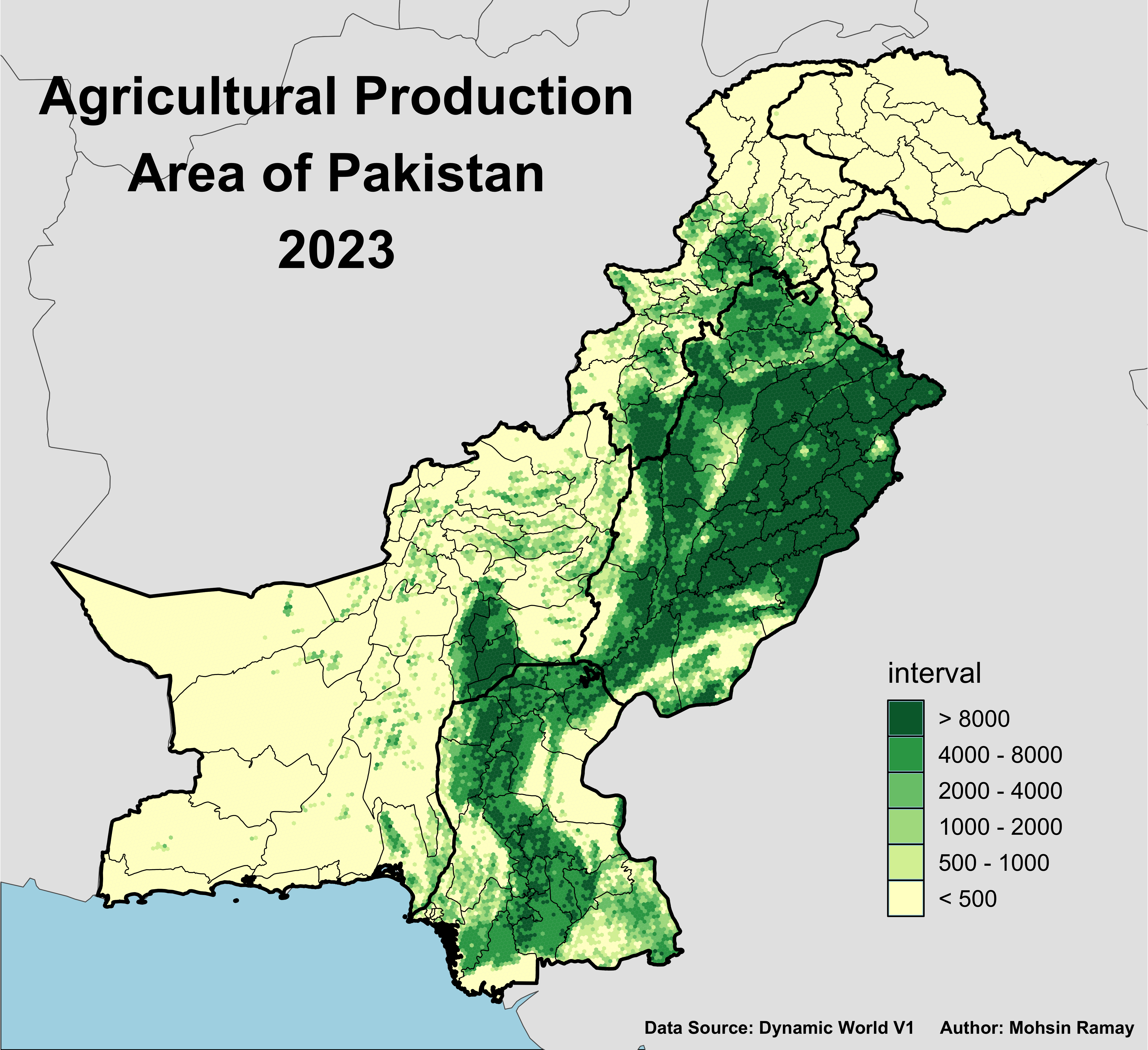

Saving the Map

To save the map with high quality, we use the ggsave function.

ggsave("Agri_Area_Pakistan_2023.png", dpi = 400, width = 7.65, height = 7)

Conclusion

This blog post demonstrated how to calculate and visualize cropping area in Pakistan using the ggplot2 package in R. The dataset used was derived from the Dynamic World V1 dataset, which offers high-resolution data for precise agricultural mapping.

The spatial map created provides insights into the distribution of agricultural land across Pakistan, highlighting the concentration in certain regions. This visualization can serve as a valuable tool for policymakers, researchers, and stakeholders involved in agricultural planning and resource allocation.

That’s it!

Feel free to reach me out if you got any questions.

remote sensing cropping area Data Science geospatial data Pakistan