Soil Texture Mapping: Integrating Google Earth Engine and R for Precise Geospatial Analysis

Data Overview: OpenLandMap Soil Texture Class (USDA System)

The OpenLandMap dataset provides soil texture classification for six soil depths (0, 10, 30, 60, 100, and 200 cm) at a 250-meter resolution. It categorizes soils based on the USDA system, making it highly relevant for agricultural and environmental studies.

For further information on the dataset and soil texture classes, visit the dataset page.

1. Loading Boundary Data in R

We begin by loading the boundary data for Germany using the rgeoboundaries package, which offers a convenient way to obtain administrative boundaries for various countries.

# Load libraries
library(tidyverse)
library(sf)
library(terra)
library(rgeoboundaries)

# Load Germany boundary data at the country level (administrative level 0)
adm0 <- geoboundaries(country = c("Germany"))

# Load Germany boundary data at the first administrative level (e.g., regions)
adm1 <- geoboundaries(country = c("Germany"), adm_lvl = "adm1")

# Plot the geometry of administrative level 1 boundaries with a blue border
plot(st_geometry(adm1), border = "blue")

# Add the country boundary (administrative level 0) to the existing plot in bold
plot(st_geometry(adm0), add = TRUE, size = 2)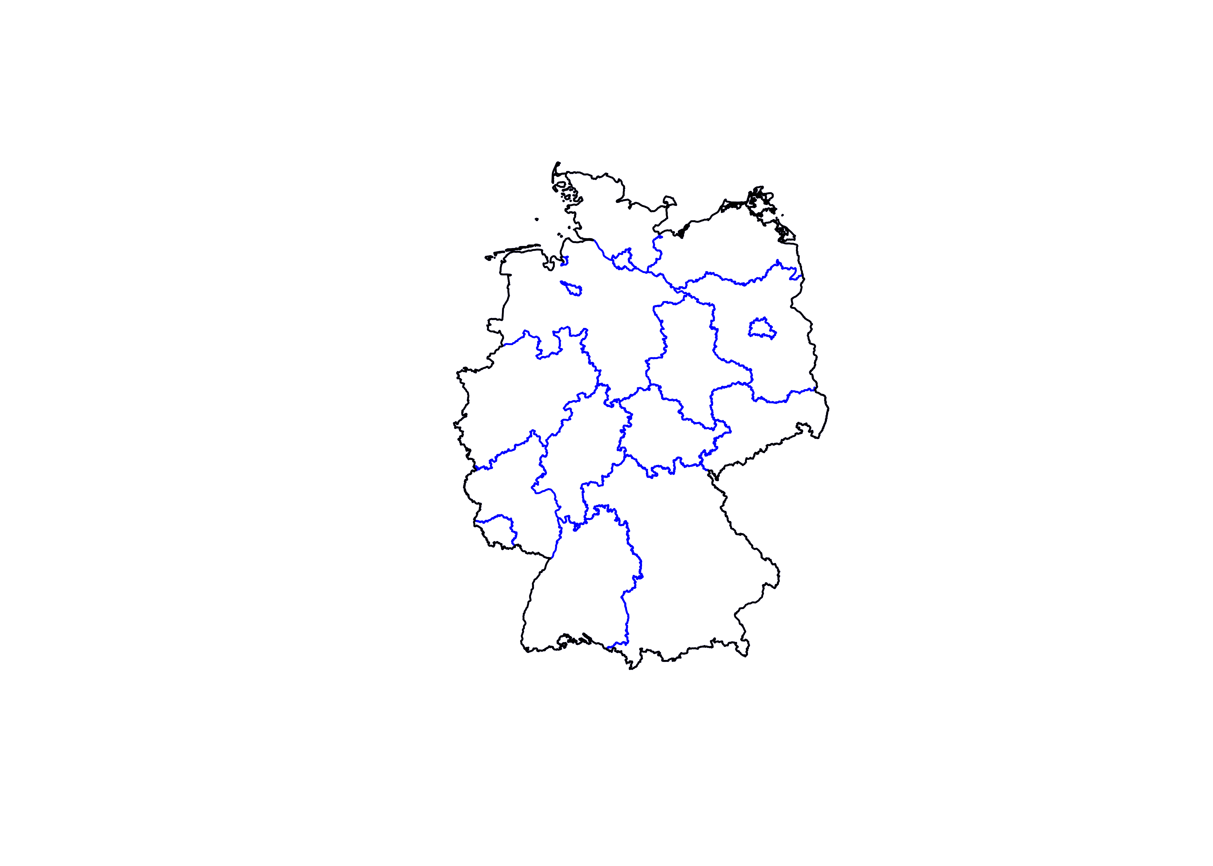

The above code snippet loads Germany’s administrative boundaries, with adm0 representing the national boundary and adm1 depicting regional divisions. These boundaries will later be used for clipping soil texture data to the relevant study area.

2. Saving Boundary Data for Google Earth Engine (GEE)

We export the country boundary (adm0) as a shapefile to use in Google Earth Engine for processing soil texture data.

# Save Germany boundary as a shapefile
adm0 |> 
  st_write("data/germany_boundary.shp")

3. Soil Texture Data Processing in GEE

Next, we use Google Earth Engine (GEE) to process the soil texture data and clip it to the German boundary. Below is the core GEE code that processes the OpenLandMap soil data.

The code can also be accessed here in the Google Earth Engine Editor.

// Define the boundary for Germany using a predefined feature collection
var germany = ee.FeatureCollection("projects/ee-mohsinramay/assets/germany_boundary");

// Load the soil texture dataset from OpenLandMap
var dataset = ee.Image('OpenLandMap/SOL/SOL_TEXTURE-CLASS_USDA-TT_M/v02');

// Clip the dataset to the boundary of Germany
var clippedDataset = dataset.clip(germany);

// Visualization parameters for the 'b0' band (soil texture classes)
var visualization = {
  bands: ['b0'],  
  min: 1.0,       
  max: 12.0,      
  palette: [
    'd5c36b', 'b96947', '9d3706', 'ae868f', 'f86714', '46d143',
    '368f20', '3e5a14', 'ffd557', 'fff72e', 'ff5a9d', 'ff005b'
  ]
};

// Center the map and add the layer
Map.centerObject(germany);
Map.addLayer(clippedDataset, visualization, 'Clipped Soil Texture');

// Export the clipped image to Google Drive
Export.image.toDrive({
  image: clippedDataset.select('b0'),
  description: 'Germany_Soil_Texture_b0',
  folder: 'Remote Sensing',
  scale: 250,
  region: germany.geometry(),
  maxPixels: 1e13
});

Instructions: After running this code in GEE, download the clipped raster data from Google Drive.

4. Bringing the Data into R for Further Processing

Once the soil texture data is downloaded, we import it into R and process it for further analysis. We align the data with Germany’s boundary and crop out any irrelevant areas.

# Load soil texture data in R
soil_text <- rast("data/Germany_Soil_Texture_b0.tif")
plot(soil_text)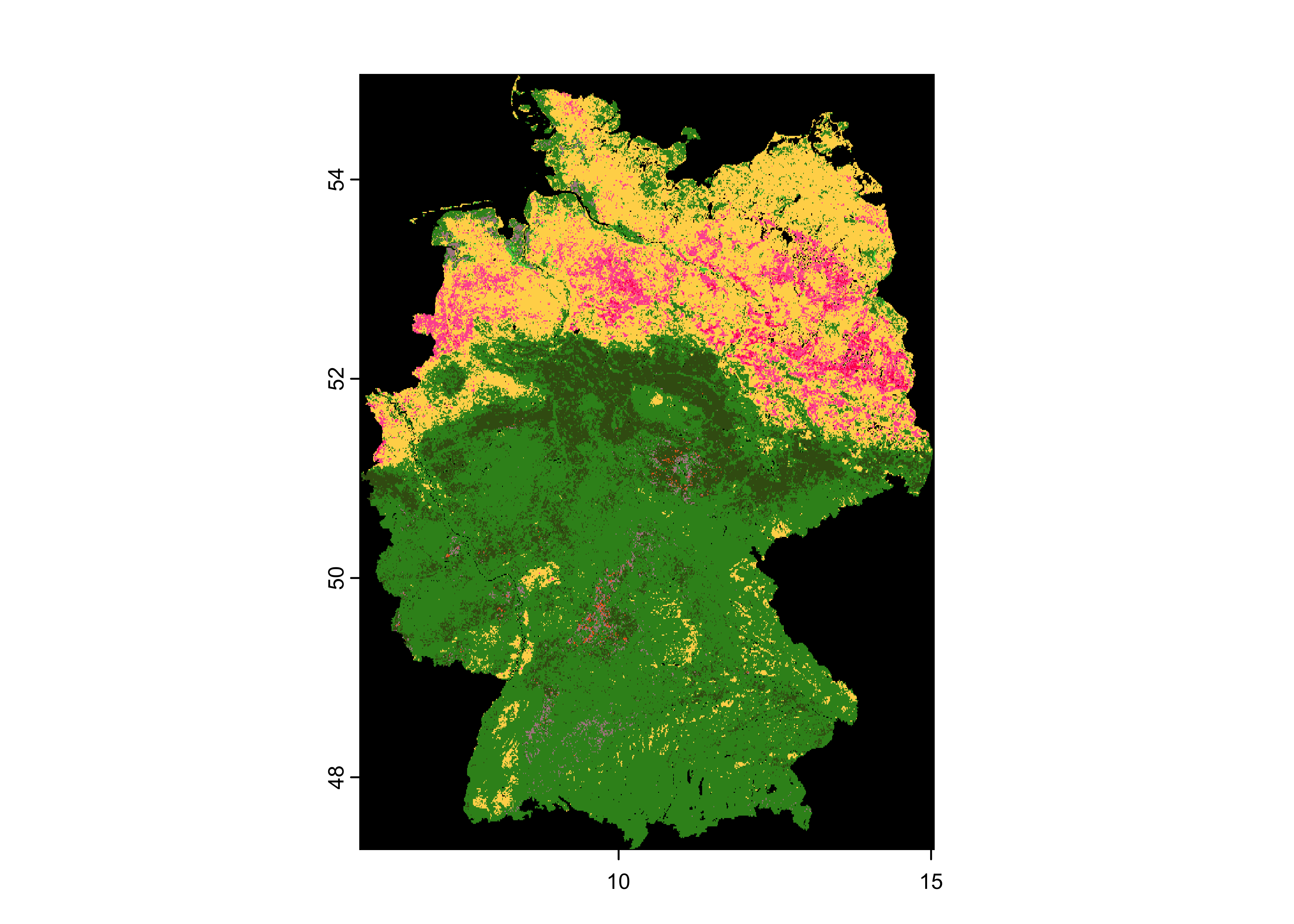

# Project soil texture data to match the CRS of Germany boundary
soil_text <- soil_text |> 
  terra::project(crs(adm0))
plot(soil_text)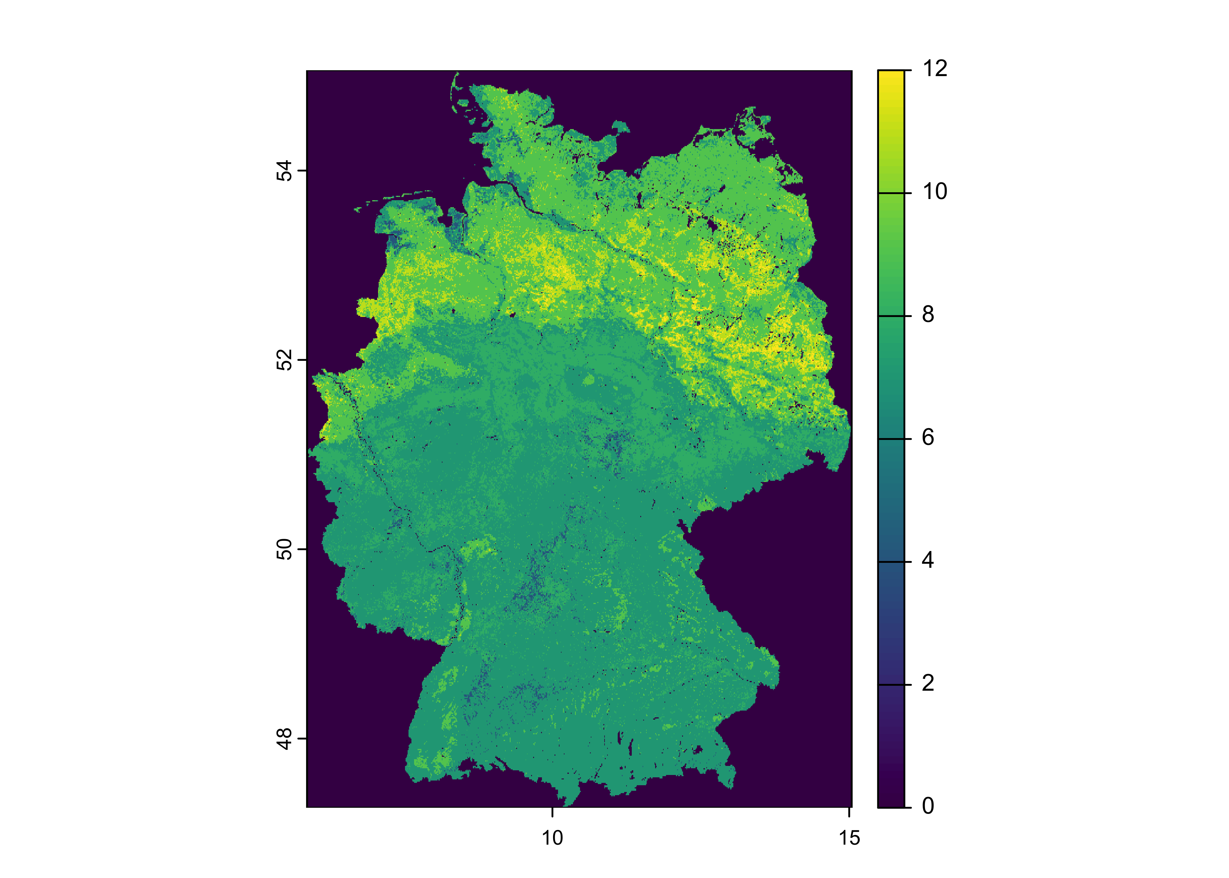

# Crop the soil texture data to the Germany boundary
soil_text_c <- terra::mask(x = soil_text, mask = adm0)
plot(soil_text_c)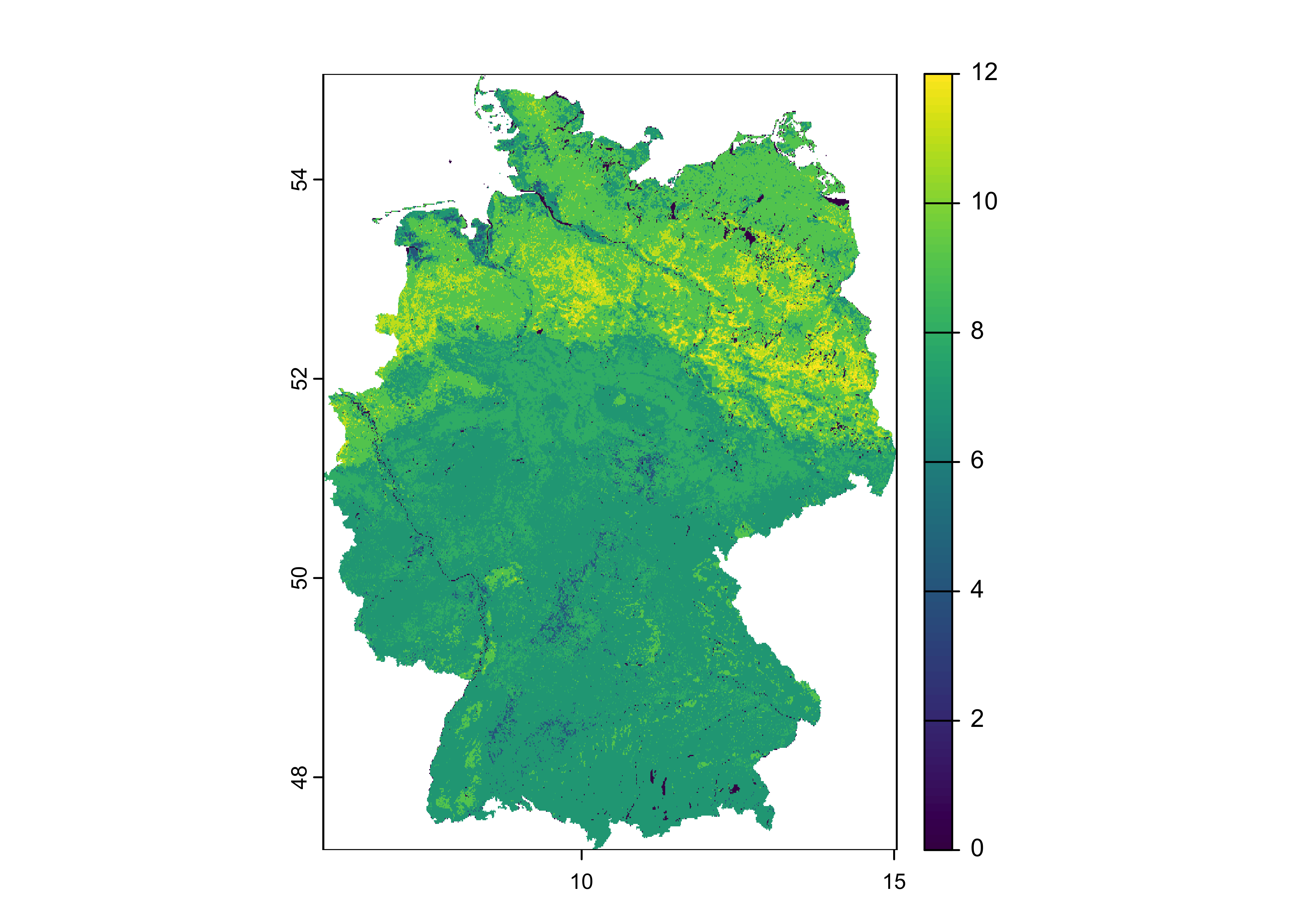

Here, the terra::project and terra::mask functions are used to align the soil texture data with the boundary of Germany and mask out areas that fall outside the country’s borders.

5. Mapping Soil Texture Colors for Visualization

To ensure the map looks professional, we manually define the colors for each soil texture class and merge this information with the processed data.

# Define soil texture classes and their corresponding colors
# This lookup table will map the 'b0' values (soil texture classes) to human-readable descriptions and assigned colors for visualization
soil_texture_lookup <- tibble(
  b0 = c(1, 2, 3, 4, 5, 6, 7, 8, 9, 10, 11, 12),  # 'b0' is the band representing soil texture types in the dataset
  description = c("Clay", "Silty Clay", "Sandy Clay", 
                  "Clay Loam", "Silty Clay Loam", "Sandy Clay Loam", 
                  "Loam", "Silty Loam", "Sandy Loam", 
                  "Silt", "Loamy Sand", "Sand"),  # Human-readable descriptions for each soil texture type
  color = c("#a6611a", "#dfc27d", "#d95f02", "#b35806", "#fee08b", 
            "#e6f598", "#66bd63", "#3288bd", "#e0f3f8", "#5e4fa2", 
            "#abdda4", "#fdae61")  # Corresponding hex color codes for each soil texture type
)

# Convert raster data to a data frame with xy coordinates for plotting
# Filter out any cells with 'b0' values of 0 (non-soil regions or NA) 
soil_data <- soil_text_c |> 
  as.data.frame(xy = TRUE) |>  # Convert raster data into a format that ggplot2 can understand
  filter(b0 != 0) |>  # Remove any invalid or zero values for soil texture classification
  left_join(soil_texture_lookup, by = "b0")  # Join the soil data with the lookup table to add soil texture descriptions and colors

This ensures that each soil texture class is mapped to a corresponding color for easier interpretation of the soil texture map.

6. Visualizing Soil Texture Data in R

We use ggplot2 to create a high-quality map of soil textures across Germany, with distinct colors representing different soil types.

pp <- soil_data |> 
  ggplot() + 
  theme_void(base_size = 14) +  # Use a minimal theme to focus on the map
  xlim(5.86625, 15.04182) +  # Set x-axis limits for Germany
  ylim(47.27012, 55.05878) +  # Set y-axis limits for Germany
  geom_raster(aes(x = x, y = y, fill = description)) +  # Plot soil texture raster data
  scale_fill_manual(values = soil_texture_lookup$color,  
                    name = "Soil Texture Class") +  # Manually assign colors to soil texture classes
  geom_sf(data = adm1, fill = NA, color = "black", linewidth = 0.75) +  # Add regional boundaries
  geom_sf(data = adm0, fill = NA, color = "black", linewidth = 0.8) +  # Add country boundary
  coord_sf() +  # Use spatial coordinates for better alignment
  theme(#legend.position = c(0.99, 0.25),  # Customize legend (position commented out)
    legend.title = element_text(size = 10, face = "bold"), 
    legend.text = element_text(size = 9, face = "bold"), 
    legend.spacing.x = unit(0.2, 'cm'), 
    legend.spacing.y = unit(0.2, 'cm')) + 
  labs(fill = "Soil Texture",  
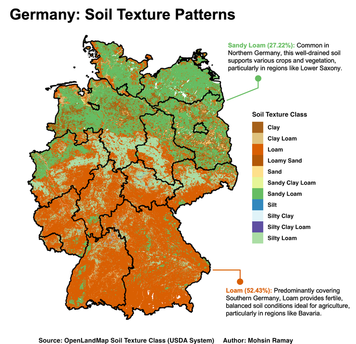
       title = "Germany: Soil Texture Patterns",  
       subtitle = "An analysis of soil texture types across Germany using OpenLandMap soil data.", 
       caption = "Source: OpenLandMap Soil Texture Class (USDA System)     Author: Mohsin Ramay") + 
  theme(plot.title = element_text(hjust = 0.5, face = "bold"), 
        plot.subtitle = element_text(hjust = 0, size = 12), 
        plot.caption = element_text(size = 10, face = "bold", hjust = -0.9))  # Center title and customize caption

pp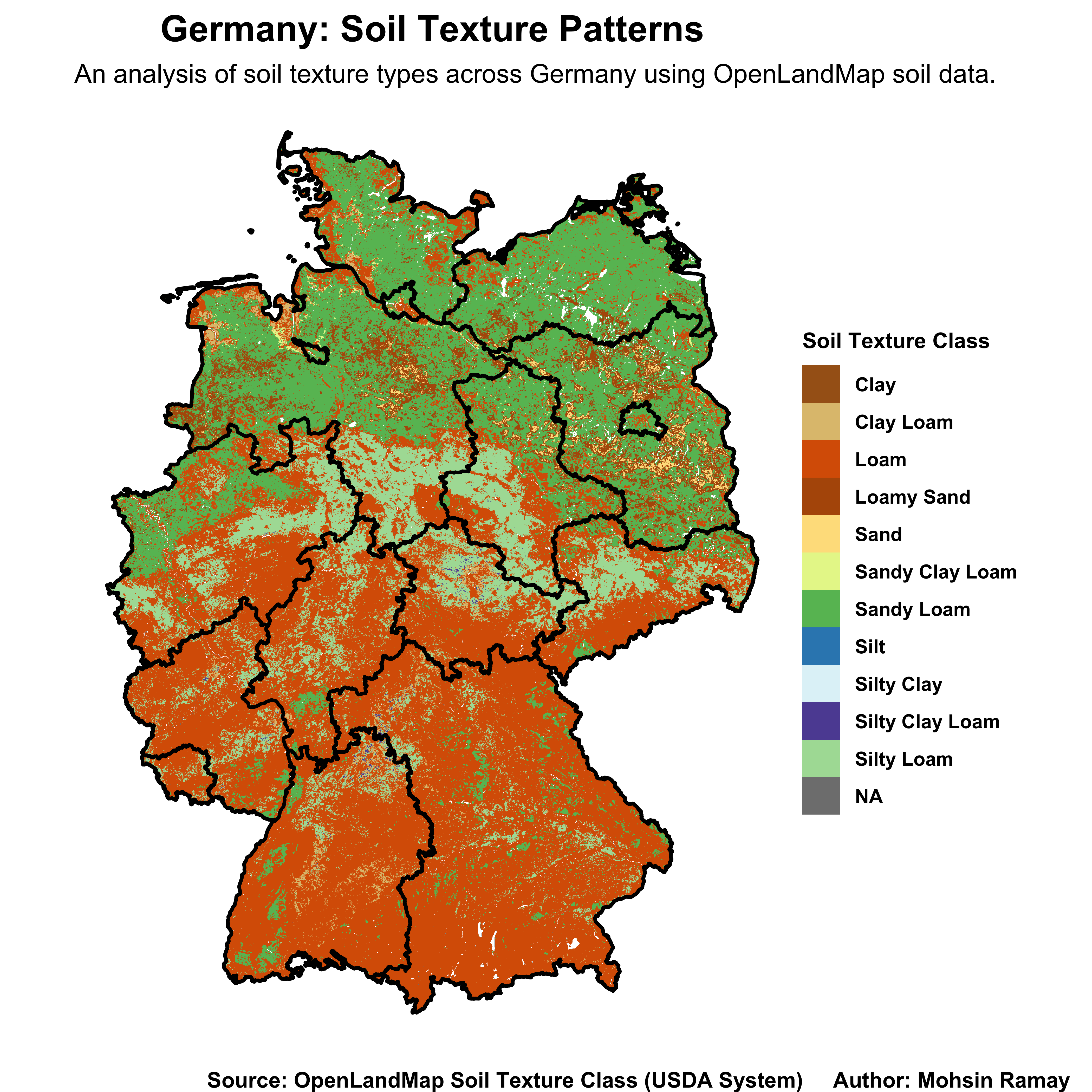

# Save the plot as a high-resolution PNG
ggsave("Final Figures/germany_soil_texture_map.jpeg", pp, dpi = 400, width = 7, height = 7)

The resulting map provides a clear and professional visualization of the soil texture distribution across Germany.

Conclusion: Key Observations from Germany’s Soil Texture Map

The map of soil textures across Germany shows distinct regional patterns. In the South and Southwestern regions, particularly in Bavaria and Baden-Württemberg, Loam dominates, providing fertile conditions for agriculture. In contrast, Sandy Loam is prevalent in the Northern regions, such as Lower Saxony and Schleswig-Holstein, where sandy soils are more common in lower-lying areas.

These soil texture patterns are influenced by Germany’s diverse topography and climate, making this type of analysis essential for agricultural and environmental management across the country.

That’s it!

Feel free to reach me out if you got any questions.